I Put TabPFN v3 Against LightGBM on Four Real Regression Problems
Code and artifacts: The complete benchmark, saved results and reproduction instructions are available in the companion GitHub repository.
Tabular foundation models are having a moment. The pitch is hard to ignore: take a pretrained model, give it a table, and get strong predictions without spending hours tuning a separate model for every problem. That sounds wonderful. It also sounds like the sort of claim that deserves a proper test.
So I put TabPFN v3 against LightGBM (my go-to model for almost every supervised learning task) on four real regression datasets. I tested clean prediction, smaller training histories, missing features, latency and API usage.
The result was not a clean victory for either side. Operationally, the gap was clearer. LightGBM scored weekly batches in milliseconds. The hosted TabPFN API took seconds and used 24.3 million measured tokens across the walk-forward experiments. That tension—strong predictions versus a more complicated deployment path—is the real story here.
First, what is TabPFN?
TabPFN stands for Tabular Prior-data Fitted Network. It is a transformer built specifically for structured data rather than text, images or audio. The project started as academic research.
Its second major version was published in Nature. TabPFN is now developed commercially by Prior Labs. Prior Labs is a research-led company focused on tabular foundation models. Its founding team includes researchers behind TabPFN and established figures in machine learning.
The company’s ambition is bigger than one classifier or regressor. It wants foundation models that can reason directly over tables and eventually combine tables with text and images.
TabPFN v3 is its current frontier model. Prior Labs offers it through an API and commercial deployment routes, while local research packages also exist for earlier or open-weight variants. The interesting part is not simply that TabPFN uses a transformer. It is how the model learns to solve a new table.
In-context learning, but for tables
Most tabular machine learning follows a familiar routine. You take one dataset, choose an algorithm, train its parameters on that dataset, validate it, tune it, and finally save the fitted model. LightGBM works this way. Each fitted model is specialised to the table it was trained on. TabPFN takes a different route.
Before it ever sees our house, bike or energy data, it is pretrained on huge numbers of synthetic datasets. Prior Labs says the current model has learned from billions of them.
Those synthetic tables represent many possible relationships: linear effects, nonlinear interactions, noisy measurements, useful features, irrelevant features and different target distributions.
Across that pretraining process, the network learns a reusable procedure for making statistical predictions. In simple terms, it is trying to “learn how to learn” a table. When we give it a real dataset, the labelled training rows become its context. The new rows are presented alongside that context, and the model predicts their targets in a forward pass.
There is no conventional task-specific optimisation of all the model weights. This is called in-context learning, or ICL. If you have used a language model, the rough analogy is few-shot prompting. You provide examples in the prompt, and the model infers what to do next without being retrained.
For TabPFN, the examples are rows and columns rather than sentences. That analogy has limits, but it captures the important idea: your training table is not teaching a fresh model from scratch. It is giving an already-trained model the context for this particular problem.
This also clears up a common misunderstanding. “No training” does not mean TabPFN ignores the training data. The labelled rows are still essential; they are consumed as context instead of weight updates. Prior Labs describes the process as applying learned priors and optimisation strategies to a new table through ICL.
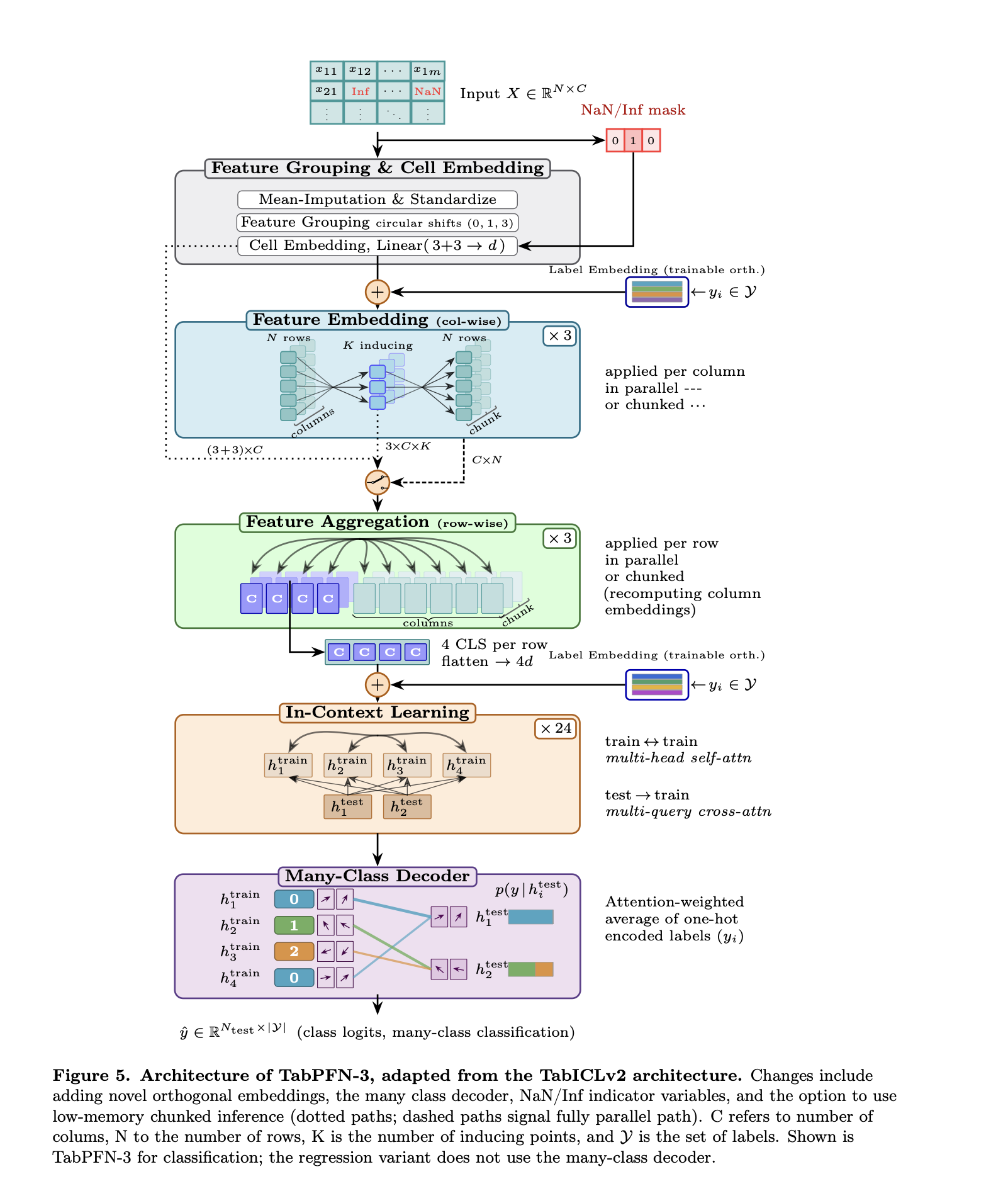
Figure 5 from the TabPFN-3 technical report. The diagram shows classification; the regression model used in this experiment does not use the final many-class decoder.
Reading from the top, TabPFN first groups features, embeds individual cells and records explicit NaN or infinity indicators. Column-wise attention learns each feature’s distribution, before row-wise aggregation compresses all columns into a fixed representation for each row.
The ICL transformer then lets training rows attend to each other, while test rows attend to the labelled training context. This is where the model infers the relationship needed for a new dataset without updating its pretrained weights.
It is an elegant idea. The practical question is whether it works better than a mature boosted-tree model on the sort of data we might actually deploy.
What I wanted to find out
I was not interested in producing another leaderboard where one MAE number decides everything. A model can win a benchmark and still be awkward, expensive or unsafe to run in production. I wanted to answer five more useful questions:
- Which model predicts the next week most accurately?
- Does that result stay consistent across several weeks?
- What happens when we remove half the historical training rows?
- What happens when important features disappear at inference time?
- What do latency, API usage and data transfer look like in practice?
The baseline was LightGBM, because it remains one of the strongest and most practical choices for tabular data. I tested two versions: a near-default 100-tree model, and a tuned model selected with 50 Optuna trials. The TabPFN entry used the official v3 API with v3_default, eight estimators, mean regression output and thinking mode disabled.
That last detail matters. This was a default ICL test, not a comparison against TabPFN’s most expensive reasoning mode.
Four datasets, four different kinds of trouble
One dataset is never enough for this sort of comparison. Models have favourite conditions, and a convenient table can make almost any method look unbeatable. I chose four public regression problems with different sizes, target shapes and deployment risks.
| Dataset | Rows | Predictors | Target | Why it is useful |
|---|---|---|---|---|
| King County house sales | 21,613 | 21 | Sale price | Spatial effects, skew and market movement |
| Seoul bike demand | 8,760 | 17 | Hourly rentals | Weather, seasonality and operating state |
| Appliances energy | 19,735 | 32 | Energy use | Correlated sensors and intraday patterns |
| Concrete strength | 1,030 | 8 | Compressive strength | A genuinely small, non-temporal table |
The house-price data came from OpenML’s King County dataset. The other three came from UCI: Seoul Bike, Appliances Energy and Concrete Strength.
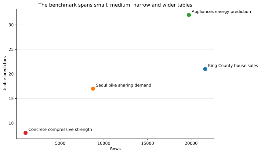
The benchmark ranges from 1,030 to 21,613 rows and from 8 to 32 usable predictors.
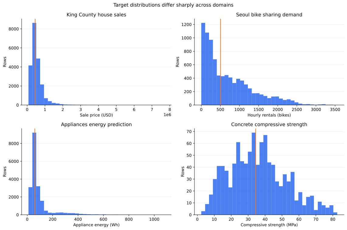
The targets are quite different too. House prices, bike rentals and appliance energy are heavily right-skewed, while Concrete strength stayed in its natural scale. I gave both model families the same log1p transform on the three skewed targets, then converted predictions back before calculating error.
Three of the four datasets also change over time. A model that performs well in March may behave differently in May.
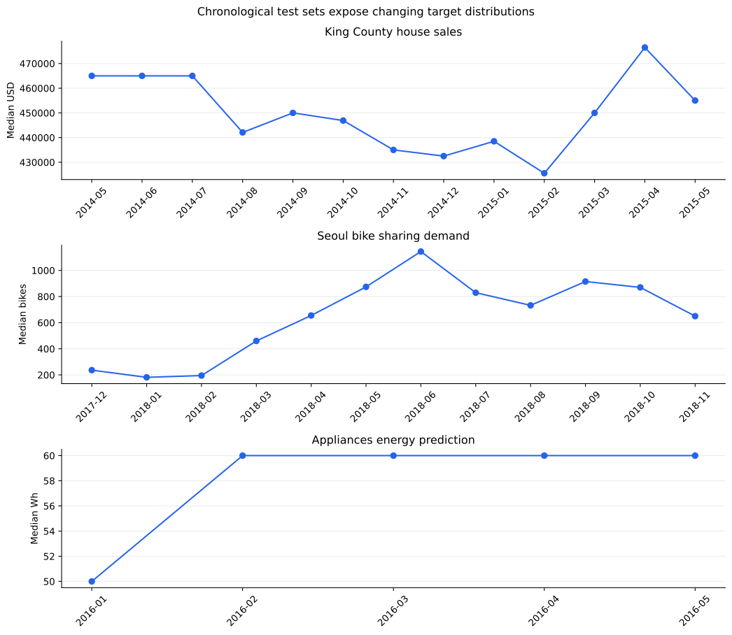
That is why the evaluation design became as important as the model choice.
The test methodology: predict one week, refit, repeat
For each dated dataset, I created eight consecutive seven-day test windows. Think of it as roughly two months of simulated deployment. Before week one, the model sees only earlier observations. It predicts the next week. Once that week is over, those labelled rows join the training history and the model is refitted. Then the process repeats.
This is usually called expanding-window walk-forward validation, or rolling-origin evaluation. It is much closer to a system that is refreshed every week. The tuned LightGBM parameters were chosen once, before the first test week. I used the preceding two weeks for validation, locked the configuration, and then refitted it on the expanding history.
TabPFN received the same expanding history as context each week. No future week influenced tuning, preprocessing or row selection. For uncertainty estimates, I resampled complete weeks rather than pretending every row was independent.
Concrete has no timestamp, so pretending it has a “next week” would be nonsense. It keeps its grouped holdout, which prevents repeated ingredient formulations from leaking between partitions.
Mean absolute error, or MAE, is the primary metric. It gives us an answer in dollars, bikes, watt-hours or megapascals rather than an abstract score. With that setup fixed, I ran three experiments.
Experiment 1: Who predicts best on clean data?
The first experiment is the clean baseline. For the dated datasets, every feature is present and each model receives all historical rows available before that week. The table combines the saved predictions from all eight test weeks; Concrete contributes its fixed grouped test result. Lower MAE is better.
| Dataset | Default LightGBM | Tuned LightGBM | TabPFN v3 | Best result |
|---|---|---|---|---|
| King County | $69,430 | $66,641 | $64,746 | TabPFN |
| Seoul Bike | 121.8 bikes | 130.6 bikes | 109.7 bikes | TabPFN numerically |
| Appliances | 54.7 Wh | 43.2 Wh | 46.2 Wh | Tuned LightGBM |
| Concrete¹ | 4.85 MPa | 4.48 MPa | 2.65 MPa | TabPFN |
¹ Concrete uses the grouped holdout rather than weekly testing.
At first glance, TabPFN wins three out of four. That summary is true, but the weekly variation and confidence intervals tell us which differences are actually convincing.
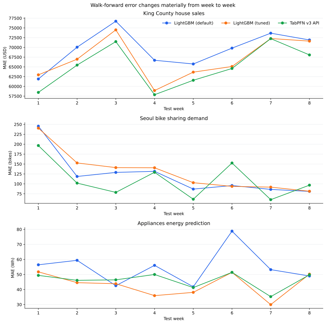
The weekly lines matter as much as the average. Performance moves around considerably.
King County: a proper TabPFN win
TabPFN produced the lowest house-price MAE at $64,746. Tuned LightGBM reached $66,641, while the default model reached $69,430. The advantage was not caused by one lucky week.
When I bootstrapped complete weeks, tuned LightGBM minus TabPFN was $1,896, with a 95% interval from $990 to $3,030. Default LightGBM minus TabPFN was $4,684, with an interval from $3,316 to $6,126. In this test, TabPFN was not merely competitive. It was reliably better.
Seoul: the average says TabPFN, uncertainty says “slow down”
TabPFN had the lowest combined Seoul MAE at 109.7 bikes. Default LightGBM followed at 121.8, with tuned LightGBM at 130.6. But TabPFN’s weekly MAE ranged from 60.2 to 196.6 bikes. That is a large swing.
The week-level interval for default LightGBM minus TabPFN ran from -12.3 to +33.6 bikes. Because it crosses zero, these eight weeks do not support a confident TabPFN win on Seoul.
Appliances: give the baseline the features it deserves
Once hour and ten-minute slot were included, tuned LightGBM won Appliances with 43.2 Wh MAE. TabPFN reached 46.2 Wh, and default LightGBM reached 54.7 Wh. The tuned LightGBM advantage over TabPFN was about 3.0 Wh. Its 95% week-level interval ran from 0.2 to 6.6 Wh, so this was a supported win rather than a rounding error.
This is a useful reminder that foundation models do not make feature design irrelevant. A strong baseline still deserves features that reflect how the underlying process works.
Concrete: where TabPFN looks most at home
Concrete is the smallest dataset, with only 1,030 rows. TabPFN reached 2.65 MPa MAE. Tuned LightGBM reached 4.48 MPa, and default LightGBM reached 4.85 MPa. That is a substantial advantage, and it fits the core appeal of TabPFN: strong predictions on small tabular problems without a long tuning exercise.
It is still a grouped, non-temporal result. It tells us nothing about drift or weekly stability, so I would not use it to make those claims.
Experiment 2: What if we have less historical data?
Foundation models are often presented as especially useful when labelled data is limited. I wanted to test that directly. For every deployment week, I kept 100%, 80%, 60% and 50% of the available historical rows. I applied the same fractions to Concrete’s grouped training partition.
The smaller samples were nested and balanced across target ranges. I repeated the temporal samples with three fixed seeds, and every model received exactly the same rows. The test weeks and Concrete test partition never changed. The 100% results are the exact clean baselines above.
This table shows MAE at 50% history divided by full-history MAE. Above 1 is worse. Below 1 means the smaller history happened to perform better.
| Dataset | Default LightGBM | Tuned LightGBM | TabPFN v3 |
|---|---|---|---|
| King County | 1.040× | 1.050× | 1.043× |
| Seoul Bike | 1.104× | 1.046× | 0.887× |
| Appliances | 0.937× | 0.992× | 0.965× |
| Concrete¹ | 1.109× | 1.107× | 1.333× |
¹ Concrete has one grouped split and one sampling seed, so treat its row-retention result more cautiously.
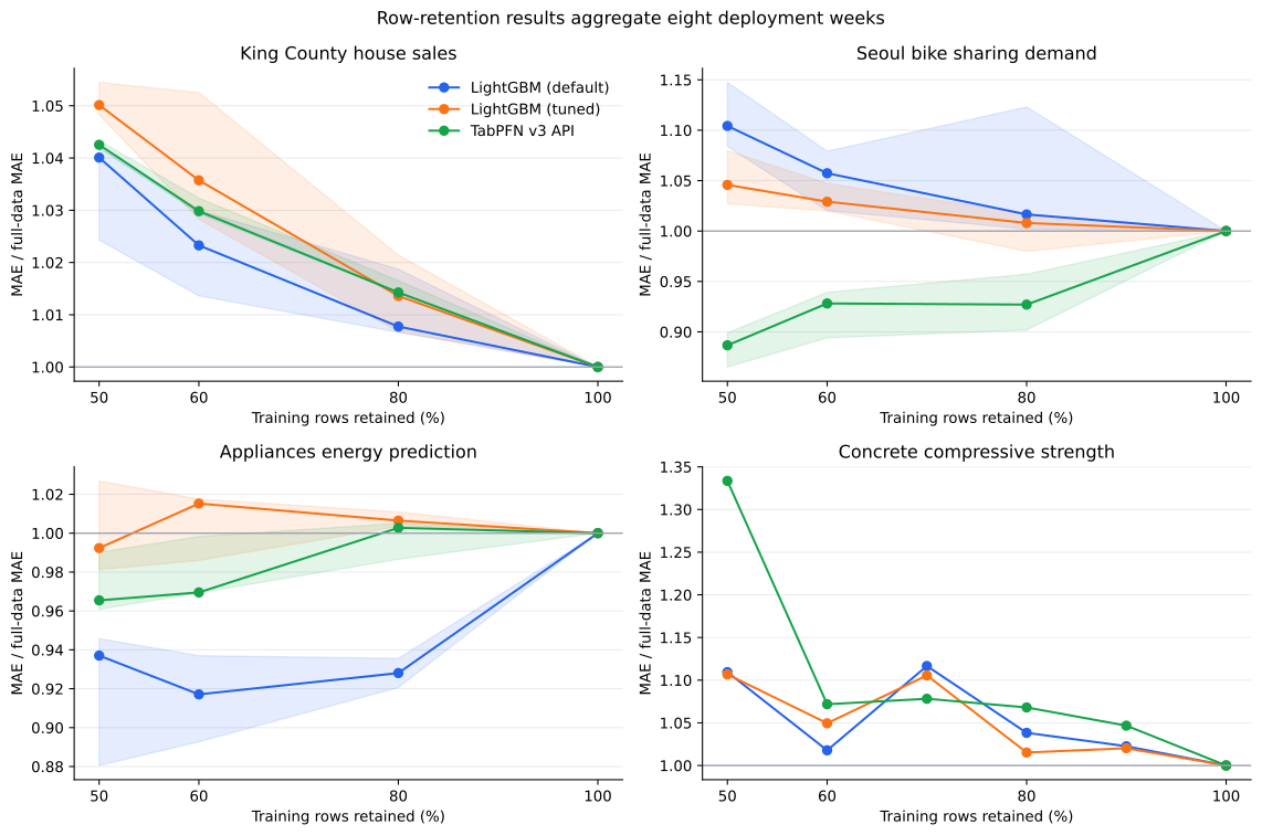
The result is messier than “less data makes every model worse”. King County behaves as expected. At half history, MAE rises by 4.0% for default LightGBM, 5.0% for tuned LightGBM and 4.3% for TabPFN.
TabPFN still has the lowest absolute MAE at roughly $67,500. Seoul does something more interesting. Both LightGBM versions get worse, while TabPFN improves across all three half-history samples. Its MAE ratio falls between 0.865 and 0.899.
Appliances is fairly stable, and several smaller histories also perform a little better. This does not mean labels are harmful. Older rows can describe stale relationships when a process is changing. A smaller sample can also act as regularisation, especially when model capacity and hyperparameters stay fixed.
The safer conclusion is that “performance degradation” is not guaranteed to be monotonic in a temporal problem. There is no universal resilience winner: TabPFN handles reduced Seoul history remarkably well, LightGBM loses less relative performance on Concrete, the models are close on King County, and Appliances barely separates them.
Absolute accuracy matters too. TabPFN loses the largest percentage on Concrete at half data, yet its resulting error is still lower than either LightGBM model.
Experiment 3: What if whole features disappear?
Real pipelines break in less polite ways than benchmark datasets. A sensor stops reporting. A join returns nulls. An upstream service changes. The model still receives a row, but one or more entire columns are missing.
I trained every model on clean history, then replaced complete test columns with missing values while keeping the schema and column order intact.
Each dated dataset-week included outages of one, three and five columns. I used five seeded combinations at each level and one predefined sequence of business-important features; Concrete received the equivalent test on its grouped partition. All models used their native missing-value handling. Every request returned valid predictions. Technically, that is 100% reliability. Predictively, the picture is much less reassuring.
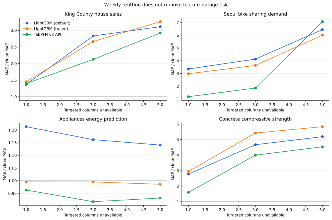
At five missing targeted columns, the MAE ratios looked like this:
| Dataset | Default LightGBM | Tuned LightGBM | TabPFN v3 |
|---|---|---|---|
| King County | 3.11× | 3.26× | 2.92× |
| Seoul Bike | 6.44× | 6.00× | 7.06× |
| Appliances | 1.14× | 0.99× | 0.93× |
| Concrete¹ | 5.18× | 5.82× | 4.53× |
¹ Concrete uses its grouped clean baseline rather than a weekly baseline.
Seoul is the clearest warning. Remove temperature, humidity, season, hour and operating state, and every model falls apart. TabPFN is actually the worst of the three. That is not a criticism of its missing-value parser. The useful information is gone. Pretraining cannot reconstruct a feature that no longer exists.
King County shows the same pattern at a smaller scale. Removing key property and location fields roughly triples error for all three models. The Appliances result looks strange again. Some outages slightly improve error for tuned LightGBM and TabPFN. I would not call that robustness.
It means some sensor relationships were unstable during these weeks, so hiding them occasionally reduced harmful extrapolation. Other seeded combinations still made error much worse.
The important production lesson is simple: accepting missing values is not the same as handling an outage safely. A real system needs freshness checks, schema validation, alerts and a fallback model trained for the degraded feature set.
The part benchmarks often skip: deployment
Accuracy was close enough that operational constraints could easily decide the model choice. LightGBM ran locally on an 8 GB Apple M2 Mac. TabPFN used Prior Labs’ hosted API.
The TabPFN timing therefore includes serialisation, upload, network transit, hosted inference and download. This is not a kernel-speed comparison. It is the end-to-end path I actually tested. The numbers below are median prediction times across the eight clean weekly batches.
| Dataset | Rows per week | Default LightGBM | Tuned LightGBM | TabPFN API |
|---|---|---|---|---|
| King County | 483 | 7.3 ms | 9.7 ms | 4.59 s |
| Seoul Bike | 168 | 6.9 ms | 9.8 ms | 2.88 s |
| Appliances | 1,008 | 6.2 ms | 6.3 ms | 3.68 s |
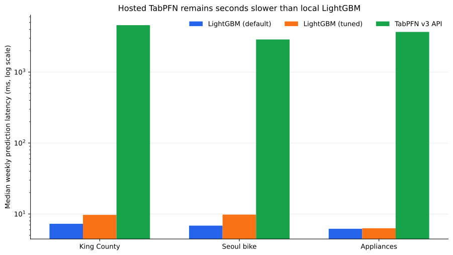
For scheduled batch scoring, a few seconds may be completely acceptable. For a user waiting on a page, a transaction or a real-time decision, it is much harder to justify—especially when local LightGBM finishes in milliseconds.
What did the API experiment use?
The TabPFN walk-forward benchmark made 504 requests, all successful, and consumed 24,323,922 measured tokens. Every returned prediction was finite.
| Dataset | Requests | Measured tokens | Cumulative API time |
|---|---|---|---|
| King County | 168 | 9,222,064 | 720.6 s |
| Seoul Bike | 168 | 2,785,894 | 490.7 s |
| Appliances | 168 | 12,315,964 | 551.3 s |
| Total | 504 | 24,323,922 | 1,762.6 s |
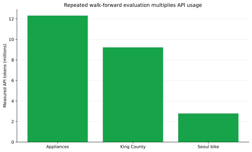
Most of that usage came from repeating the reduced-data and outage experiments. The clean weekly predictions alone used 48 requests and 2,901,875 tokens: one context-building call and one prediction call for each dataset-week.
There is no universal public dollar conversion that applies to every agreement, so I have reported measured tokens rather than inventing a cost. A company evaluating the API should apply its own plan or enterprise quote to the saved usage records. There is also a privacy boundary.
The hosted path uploads training features, training targets and inference rows. That may be fine for public or low-sensitivity data. It may be unacceptable for customer, health or financial data without the right controls.
Prior Labs also advertises private deployment options. Those could change the latency, privacy and cost picture, but they are not what I tested here. LightGBM stayed offline and local throughout.
So, is TabPFN v3 ready for industry?
Yes—but with an asterisk large enough to deserve its own paragraph. TabPFN is ready to be taken seriously as an industrial challenger.
It recorded the lowest MAE on three of the four datasets: King County, Seoul and Concrete. The King County and Concrete wins were clear; Seoul was a numerical win with much greater week-to-week uncertainty.
That is impressive without task-specific tuning. It is not yet an automatic replacement for LightGBM.
| Dimension | LightGBM | TabPFN v3 API |
|---|---|---|
| Predictive quality | Won Appliances; competitive elsewhere | Lowest MAE on King County, Seoul and Concrete; Seoul was less conclusive week to week |
| Smaller-data behaviour | Dataset-dependent | Dataset-dependent; excellent on reduced Seoul history |
| Feature outages | No consistent protection | No consistent protection |
| Latency | Millisecond local batches | Multi-second hosted requests |
| Data control | Local and offline | Tested path uploads context and inference data |
| Tuning | Useful on Appliances, harmful on Seoul | No task-specific search in this test |
| Operations | Mature and easy to package | Hosted dependency, tokens and service behaviour |
| Licence | MIT | Depends on the chosen service or model agreement |
If I were building a high-volume synchronous service, I would still begin with LightGBM. It is fast, cheap to run, easy to keep local, and supported by a mature ecosystem. It is also a very strong baseline, as the Appliances result shows.
For a high-value batch problem with a modest-sized table, I would absolutely test TabPFN. If a $1,900 reduction in weekly house-price MAE has real business value, a few seconds of API latency may be a sensible trade.
What I took away from the experiment
The most valuable result was not that TabPFN recorded the lowest MAE on three datasets or that tuned LightGBM won Appliances. It was seeing how both behaved across eight consecutive deployment weeks rather than reducing the comparison to one score.
Across the benchmark:
- TabPFN was reliably best on King County.
- TabPFN remained exceptionally strong on the small grouped Concrete dataset.
- Tuned LightGBM was reliably best on Appliances.
- TabPFN recorded the lowest overall Seoul MAE, although eight weeks did not provide enough evidence for a confident week-level winner.
- Neither family was universally resilient to fewer rows or missing features.
My practical conclusion is straightforward.
TabPFN v3 is ready to challenge a serious tabular baseline. LightGBM is still the safer default production system.
The right choice depends on what your system values: a little more accuracy, millisecond latency, offline control, simple operations, or graceful failure. And whichever model you choose, test it in the cadence and failure modes it will actually face. That part matters more than the logo on the model.